Examples
This page contains instructions for running the Simbelmynë examples, assuming that the code has already been installed.
All the necessary scripts are in SBMY_ROOT/examples/. Typing make runs all the example of this page. At any point, one can restore a clean state by typing make clean.
Setting up the run
The script example_setup.py contains the configuration and can be adjusted (see the parameter file for a description of all the input parameters):
L0=L1=L2=250.
corner0=corner1=corner2=-125.
N0=N1=N2=128
Np0=Np1=Np2=128
Npm0=Npm1=Npm2=128
N_CAT=1
cosmo={'h':0.6774, 'Omega_r':0., 'Omega_q':0.6911, 'Omega_b':0.0486, 'Omega_m':0.3089, 'm_ncdm':0., 'Omega_k':0., 'tau_reio':0.066, 'n_s':0.9667, 'sigma8':0.8159, 'w0_fld':-1., 'wa_fld':0., 'k_max':10.0, 'WhichSpectrum':"EH"}
The default setup will result in simulations that run easily on a standard laptop.
Preparing the inputs
Generating the parameter files
The first preparatory step is to generate the parameter files for the examples runs, using python. To do so, type make parfiles, or equivalently, run the python script setup_parfiles.py.
The following files are written as a result: example_lpt.sbmy, example_pm.sbmy, example_tcola.sbmy, example_rsd.sbmy, example_mock.sbmy.
Generating the input power spectrum
The second preparatory step is to compute the initial power spectrum to be used in the simulations, given the cosmological parameters and prescription specified in example_setup.py. This is achieved by typing make power or running the python script setup_power.py. The Fourier space k-binning to be used for final power spectra is also computed.
The following files are written as a result: input_power.h5 and input_ss_k_grid.h5.
Generating the survey geometry
The third preparatory step is to prepare a simple synthetic survey geometry. To do so, type make survey or equivalently, run the python script setup_survey_geometry.py.
The following file is written as a result: input_survey_geometry.h5.
Running the simulations
We are now ready to run the actual simulations using the Simbelmynë executable. This is achieved by typing make sims or running the python script run_examples.py, which essentially executes the following commands:
pySbmy("example_lpt.sbmy", "logs_lpt.txt")
pySbmy("example_pm.sbmy", "logs_pm.txt")
pySbmy("example_tcola.sbmy", "logs_tcola.txt")
pySbmy("example_rsd.sbmy", "logs_rsd.txt")
pySbmy("example_mock.sbmy", "logs_mock.txt")
All the simulations start from the same initial conditions, generated by the first command and stored as initial_density.h5. The first run uses Lagrangian perturbation theory (LPT), the second uses a Particle-Mesh code, and the third uses tCOLA. The output density contrast fields are respectively lpt_density.h5, final_density_pm.h5, and final_density_tcola.h5. The fourth simulation uses tCOLA a forward model and additionnally puts dark matter particles in redshift space. The last simulation takes as input this redshift-space dark matter field (rs_density_tcola.h5) to produce a synthetic catalog (output_mock_c0_n0.h5) and compute its power spectrum as a summary statistic (output_ss.h5).
For the LPT run, dark matter particles are also stored in the file lpt_particles.gadget3 (in GADGET HDF file format, see the user guide for GADGET).
The logs can be checked in the corresponding files (logs_*.txt).
Displaying the density fields
The command make slices uses the tool slice to display the density contrast in logarithmic scale (i.e. \(\log(1+\delta)\)). The result should look like this:
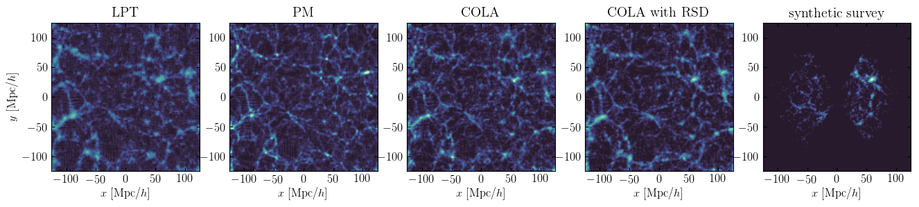
Simbelmynë examples: from left to right: dark matter density evolved with LPT, dark matter density evolved with PM, dark matter density evolved with tCOLA, dark matter density evolved with tCOLA in redshift space, synthetic galaxy catalog.
Computing and plotting final power spectra
Using the outputs, the command make test_power (or directly the script test_power.py) produces a pdf plot of power spectra of the various fields, and a plot of dark matter power spectra divided by the linear power spectrum. The result should look like this:
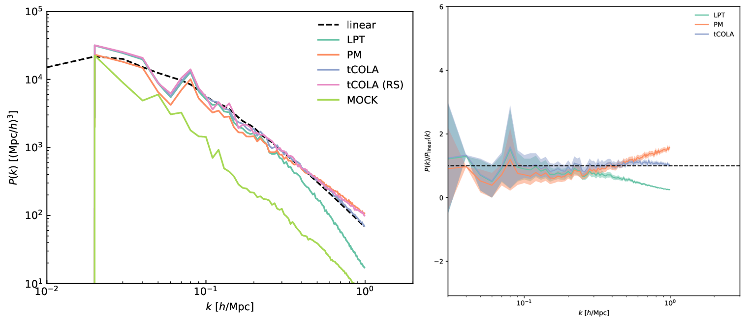
Simbelmynë examples: left: power spectra of various fields; right: dark matter power spectra divided by the linear power spectrum.